Living Without Atomic Clocks

The world’s first caesium-133 atomic clock (1955), and otherwise unrelated everything else here.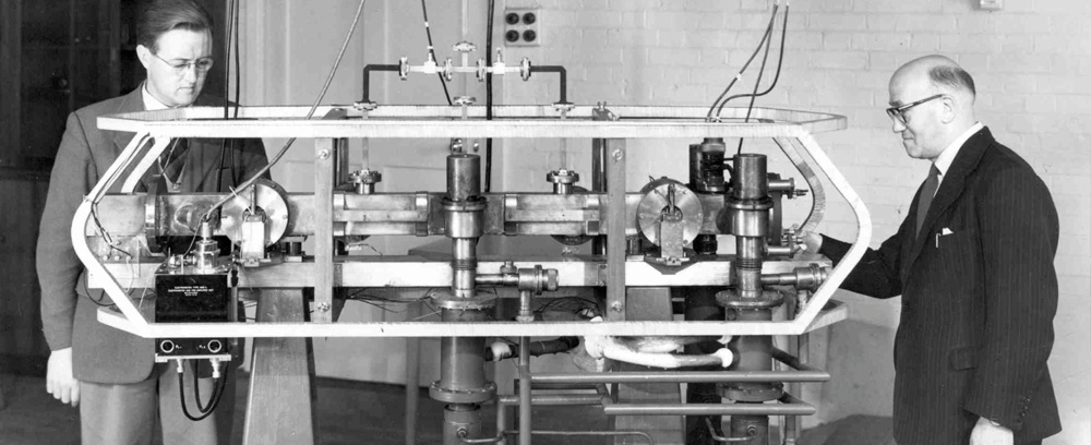

This was originally authored by Spencer Kimball about four years ago; I tried re-writing it to understand it better. You’ll also find it on our company engineering blog. To keep up with new writing, sign up for my (entirely inactive) newsletter.

One of the more inspired facets of Spanner¹ comes from its use of atomic clocks to give participating nodes really accurate wall time synchronization. The designers of Spanner call this TrueTime, and it provides a tight bound on clock offset between any two nodes in the system. This lets them do pretty nifty things! We’ll elaborate on a few of these below, but chief among them is their ability to leverage tightly synchronized clocks to provide a high level of external consistency (we’ll explain what this is too).

Seeing as how CockroachDB² (abbrev. CRDB) is supposedly the open source Spanner, for folks even remotely familiar with Spanner internals a reasonable ask at this point is something along the lines of ‘you can’t be using atomic clocks if you’re building an open source system, so how does CRDB even work?’

It’s a good question, and one we (try) to elaborate on here. As a Spanner-derived system, our challenges lie in providing similar guarantees of external consistency without having these magical clocks at hand. CRDB was intended to be run on off-the-shelf commodity hardware, on any arbitrary collection of nodes. It’s cloud neutral in that it can very well span multiple public and/or private clouds using your flavor-of-the-month virtualization layer. It’d be a showstopper to require an external dependency on specialized hardware for clock synchronization.

So what does CRDB do instead? Well, before answering that question, let’s dig a little deeper into why TrueTime was conceived for Spanner in the first place.

1. Time in Distributed Systems

Time is a fickle thing. For readers unfamiliar with the complexities around time in distributed systems research, the thing to know about it all is this: each node in the system maintains its own view of time, usually powered by its own on-chip clock device. This clock device is rarely ever going to be perfectly in sync with other nodes in the system, and as such, there’s no absolute time to refer to.

Existentialism aside, perfectly synchronized clocks are a holy grail of sorts for distributed systems research. They provide, in essence, a means to absolutely order events, regardless of which node an event originated at. This can be especially useful when performance is at stake, allowing subsets of nodes to make forward progress without regard to the rest of the cluster (seeing as every other node is seeing the same absolute time), while still maintaining global ordering guarantees. Our favorite Turing award winner has written a few words on the subject³.

2. Linearizability

By contrast, systems without perfectly synchronized clocks (read: every system) that wish to establish a complete global ordering must communicate with a single source of time on every operation. This was the motivation behind the timestamp oracle as used by Google’s Percolator⁴. A system which orders transactions \(T_1\) and \(T_2\) in the order \([T_1, T_2]\) provided that \(T_2\) starts after \(T_1\) finishes, regardless of observer, provides for the strongest guarantee of consistency called external consistency⁵. To confuse things further, this is what folks interchangeably refer to as linearizability or strict serializability. Andrei has more words on this soup of consistency models here.

3. Serializability

Let’s follow one more tangent and introduce the concept of serializability. Most database developers are familiar with serializability as the highest isolation level provided by the ANSI SQL standard. It guarantees that the constituent reads and writes within a transaction occur as though that transaction were given exclusive access to the database for the length of its execution, guaranteeing that no transactions interfere with each other. In other words, no concurrent transaction \(T_2\) is able to read any partially-written state of transaction \(T_1\) or perform writes causing transaction \(T_1\) to read different values for the same key over the course of its execution.

In a non-distributed database, serializability implies linearizability for transactions because a single node has a monotonically increasing clock (or should, anyway!). If transaction \(T_1\) is committed before starting transaction \(T_2\), then transaction \(T_2\) can only commit at a later time.

In a distributed database, things can get dicey. It’s easy to see how the ordering of causally-related transactions can be violated if nodes in the system have unsynchronized clocks. Assume there are two nodes, \(N_1\) and \(N_2\), and two transactions, \(T_1\) and \(T_2\), committing at \(N_1\) and \(N_2\) respectively. Because we’re not consulting a single, global source of time \(t\), transactions use the node-local clocks to generate commit timestamps \(ts\). To illustrate the trickiness around this stuff, let’s say \(N_1\) has an accurate one but \(N_2\) has a clock lagging by \(100ms\). We start with \(T_1\), addressing \(N_1\), which is able to commit at \(ts = 150ms\). An external observer sees \(T_1\) commit and consequently starts \(T_2\), addressing \(N_2\), \(50ms\) later (at \(t = 200ms\)). Since \(T_2\) is annotated using the timestamp retrieved from \(N_2\)’s lagging clock, it commits in the past, at \(ts = 100ms\). Now, any observer reading keys across \(N_1\) and \(N_2\) will see the reversed ordering, \(T_2\)’s writes (at \(ts = 100ms\)) will appear to have happened before \(T_1\)’s (at \(ts = 150ms\)), despite the opposite being true. ¡No bueno! (Note that this can only happen when the two transactions access a disjoint set of keys.)

Causally related transactions committing out of order due to unsynchronized clocks.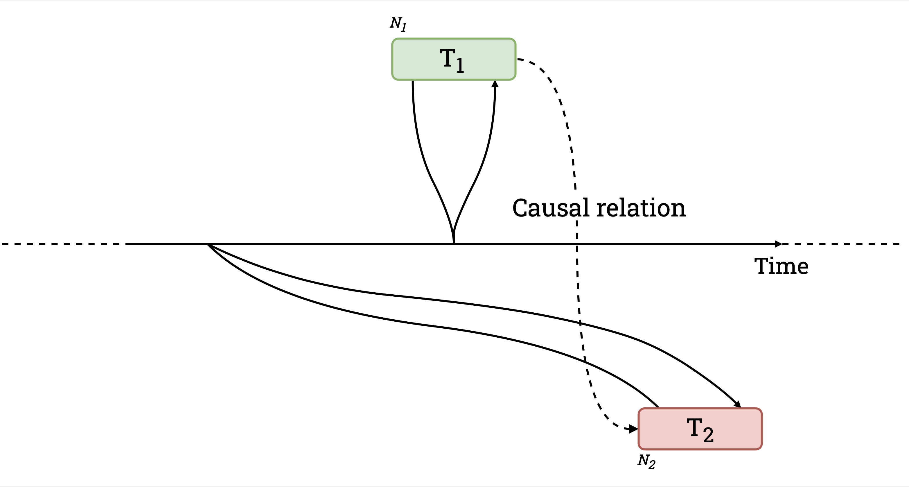

The anomaly described here, and shown in the figure above, is something we call causal reverse. While Spanner provides linearizability, CRDB only goes as far as to claim serializability, though with some features to help bridge the gap in practice. I’ll (lazily) defer to Andrei again, he really does cover a lot of ground here.

4. How does TrueTime provide linearizability?

So, back to Spanner and TrueTime. It’s important to keep in mind that TrueTime does not guarantee perfectly synchronized clocks. Rather, TrueTime gives an upper bound for clock offsets between nodes in a cluster. The use of synchronized atomic clocks is what helps minimize the upper bound. In Spanner’s case, Google mentions an upper bound of 7ms. That’s pretty tight; by contrast, using NTP for clock synchronization is likely to give somewhere between 100ms and 250ms.

So how does Spanner use TrueTime to provide linearizability given that there are still inaccuracies between clocks? It’s actually surprisingly simple. It waits. Before a node is allowed to report that a transaction has committed, it must wait 7ms. Because all clocks in the system are within 7ms of each other, waiting 7ms means that no subsequent transaction may commit at an earlier timestamp, even if the earlier transaction was committed on a node with a clock which was fast by the maximum 7ms. Pretty clever.

Careful readers will observe that the whole wait out the uncertainty idea is not predicated on having atomic clocks lying around. One could very well wait out the maximum clock offset in any system and achieve linearizability. It would of course be impractical to have to eat NTP offsets on every write, though perhaps recent research⁶ in this area may help bring that down to under a millisecond.

Fun fact: early CRDB had a hidden –linearizable switch that would do essentially the above, so theoretically, if you did have atomic clocks lying around (or generally an acceptable maximum clock offset), you’d get Spanner-like behavior out of the box. We’ve since removed it given how under-tested it was, but perhaps it would make sense to resurrect it as cloud providers trend towards exposing TrueTime-like APIs. Chip-scale atomic clocks are a reality; putting one on server motherboards would beat the pants off a quartz crystal oscillator.

5. How important is linearizability?

Stronger guarantees are a good thing, but some are more useful than others. The possibility of reordering commit timestamps for causally related transactions is likely a marginal problem in practice. What could happen is that examining the database at a historical timestamp might yield paradoxical situations where transaction \(T_1\) is not yet visible while transaction \( T_2\) is, even though transaction \(T_1\) is known to have preceded \(T_2\), as they’re causally related. However, this can only happen if (a) there’s no overlap between the keys read or written during the transactions, and (b) there’s an external low-latency communication channel between clients that could potentially impact activity on the database.

For situations where reordering could be problematic, CRDB makes use of a causality token, which is just the maximum timestamp encountered during a transaction. It’s passed from one actor to the next in a causal chain, and serves as a minimum timestamp for successive transactions to guarantee that each has a properly ordered commit timestamp. Of course, this mechanism doesn’t properly order independent causal chains, though imagining a use case where that’s a problem requires creativity.

But there’s a more critical use for TrueTime than ordering transactions. When starting a transaction reading data from multiple nodes, a timestamp must be chosen which is guaranteed to be at least as large as the highest commit time across all nodes. If that’s not true, then the new transaction might fail to read already-committed data – an unacceptable breach of consistency. With TrueTime at your disposal, the solution is easy; simply choose the current TrueTime. Since every already-committed transaction must have committed at least 7ms ago, the current node’s wall clock must have a time greater than or equal to the most recently committed transaction. Wow, that’s easy and efficient. So what does CRDB do?

6. How does CockroachDB choose transaction timestamps?

The short answer? Something not as easy and not as efficient. The longer answer is that CRDB discovers an appropriate timestamp for the transaction as it proceeds, sometimes restarting it at a later timestamp if needed.

As mentioned earlier, the timestamp we choose for the transaction must be greater than or equal to the maximum commit timestamp across all nodes we intend to read from. If we knew the nodes which would be read from in advance, we could send a parallel request for the maximum timestamp from each and use the latest. But this is a bit clumsy, since CRDB was designed to support conversational SQL where the read/write sets are indeterminate, we can’t know the nodes in advance. It’s also inefficient because we would have to wait for the slowest node to respond before even starting execution. Aside: readers may be interested in Calvin⁷ and SLOG⁸, a family of research systems developed around declaring read/write sets upfront (though giving up conversational SQL) which consequently manages to avoid this class of problems.

What CRDB does instead is actually surprisingly similar to what Spanner does, though with much looser clock synchronization requirements. Put simply:

While Spanner always waits after writes, CockroachDB sometimes waits before reads.

When CRDB starts a transaction, it chooses a provisional commit timestamp based on the current node’s wall time. It also establishes an upper bound on the selected wall time by adding the maximum clock offset for the cluster. This time interval, \([\ \mathit{commit\ ts}, \mathit{commit\ ts} + \mathit{max\ clock\ offset}\ ]\), represents the window of uncertainty.

As the transaction reads data from various nodes, it proceeds without difficulty so long as it doesn’t encounter a key written within this interval. If the transaction encounters a value at a timestamp below its provisional commit timestamp, it trivially observes the value during reads and overwrites the value at the higher timestamp during writes. It’s only when a value is observed to be within the uncertainty interval that CRDB-specific machinery kicks in. The central issue here is that given the clock offsets, we can’t say for certain whether the encountered value was committed before our transaction started. In such cases, we simply make it so by performing an uncertainty restart, bumping the provisional commit timestamp just above the timestamp encountered. Crucially, the upper bound of the uncertainty interval does not change on restart, so the window of uncertainty shrinks. Transactions reading constantly updated data from many nodes may be forced to restart multiple times, though never for longer than the uncertainty interval, nor more than once per node.

As mentioned above, the contrast between Spanner and CRDB is that Spanner always waits on writes for a short interval, whereas CRDB sometimes waits on reads for a longer interval. How long is that interval? Well, it depends on how clocks on CRDB nodes are being synchronized. Using NTP, it could very well be up to 250ms. Not great, but the kind of transaction that would restart for the full interval would have to be reading constantly updated values across many nodes. These kinds of patterns do exist in practice, but are the exception.

Because CRDB relies on clock synchronization, nodes periodically compare clock offsets amongst themselves. If the configured maximum offset is exceeded by any node, it self-terminates. If you’re curious about what happens when maximum clock offsets are violated, we’ve thought about it a bit here.

8. Concluding thoughts

If you’ve made it this far, thanks for hanging in there. If you’re new to it all, this is tricky stuff to grok. Even we occasionally need reminding about how it all fits together, and we built the damn thing.